The Use of Plant Characterisation Modelling Studies to Substantiate National Conservation and Sustainability Policies
 James Furze
University of the West of England, Faculty of Environment and Technology
James.Furze@uwe.ac.uk
.
 Quanmin Zhu
Professor at University of the West of England, Faculty of Environment and Technology
Quan.Zhu@uwe.ac.uk
.
 Jennifer Hill
Associate Professor at University of the West of England, Faculty of Environment and Technology
Jennifer.Hill@uwe.ac.uk
[soundcloud url=”http://api.soundcloud.com/tracks/106152548″ params=”” width=” 100%” height=”166″ iframe=”true” /]
Abstract: Plant characterisation is key to the study of biodiversity. It is multidisciplinary and includes historical, biogeographical, scientific and mathematic elements. Modelling of plant species has been carried out with qualitative use of the water-energy dynamic. Quantitative measurements of plant characterisation are essential to biodiversity, sustainability and conservation policy formation of local, national and global areas. Characteristics of plants are plant life-history strategies, photosynthetic type and life-forms. In the Species-Area relationship locations of high biodiversity are examined in terms of the number of species in each location and subjected to a regression of values according to the relationship of increasing numbers of species with increasing area. Subsequently an algorithmic breakdown of the climatic and topographic conditions is carried out according to T-S-K fuzzy logic, variables are specified and given definition in the example location of Guyana, South America. A genetic-dispersal of the elements of plant strategies is carried out, elements are plotted on combined objective axis, showing a Pareto distribution which may be extrapolated to alternate scales. The results show the following: individual occurrences of plant species versus locations of high biodiversity, the Species-Area relationship with statistical testing. Data are shown and an algorithm is detailed. A summary table of the ordination of plant species in seven environments is shown. The rule-base for the stress tolerant-ruderal strategy environment of Guyana is given and a 3-dimensional surface area plot of minimized elements is presented. The plant strategy Pareto is plotted and rules structuring the combined objective space are provided. In conclusion the Species-Area relationship does not explain the increase of species numbers and a descriptive form of ordination is required to cater for variable conditions, determining individual species occurrence. T-S-K modelling allocates environments to example locations with a global spread and predicts the occurrence of plant species. The conditions determining plant characteristics may be minimized to contain essential elements (mean temperature and precipitation) of the water-energy dynamic. The structure of T-S-K fuzzy logic enables genetic mathematic technique to be employed, allowing enhanced prediction of climatic variables and additionally of species numbers. Plant characterisation modelling studies strengthen national conservation and sustainability policies key to ecosystems and developing human communities which are dependent upon them.
Keywords: Plant characterisation, modelling, Species-Area, algorithmic, genetic dispersal, water-energy dynamic, conservation and sustainability policies.
.
Introduction
Studies and different approaches to quantify species within ecology and in different geographical locations trace back to the beginnings of scientific endeavour and civilisation itself (Humboldt, 1806, Schultes and Reis, 1997). We include classical, historical and modern approaches to the subject. The nature of plant characterisation is multidisciplinary, consists of many different subject areas and generative in producing new areas of study. It would be difficult to provide complete reference of all areas, which benefitting progress within the subject, the author provides background of areas, which provide the current approach and progress within the subject.
Humboldt (1845-1858) became the first to predict the Chocó region and Andean forests as one of the mega centres of plant diversity:
‘Die dem Äquator nahe Gebirgsgegend … von Neugranada [today: Columbia] … ist der Teil der Oberfläche unseres Planeten, wo im engsten Raum die Mannigfaltigkeit der Natureindrücke [today: biodiversity] ihr Maximum erreicht’ (Humboldt, 1845, p. 12) (English translation by Otté(1860, p. 10): ’… The countries bordering on the equator[meant is the present-day country of Colombia] possess another advantage … This portion of the surface of the globe affords in the smallest space the greatest possible variety of impressions from the contemplation of nature[today: biodiversity]’ (Barthlott, Mutke, Rafiqpoor, Kier and Kreft, 2005).
Remarkably Humboldt hypothesized explanations for diversity including complex topography and climatic conditions in the Chocó region (Humboldt, 1808), Humboldt provided the initial statements which substantiate the water-energy dynamic (Wright, 1983), Humboldt speculated that plant richness declines at higher latitudes due to the fact that many species are frost intolerant and may not survive in the comparatively cooler temperatures of temperate zone winters. Wright surmises that plant productivity is limited by energy from the sun and water availability, however the solar energy that transfers through each trophic level is what constrains richness as opposed to the total energy within a geographic area – the productivity hypothesis (Wright, 1983; Hawkins et al., 2003; Jetz, Kreft, Ceballos, and Mutke, 2009).
Quantitative measurements of species characteristics are key in biodiversity, conservation and potential sustainability policies. Numbers of species per unit area is fundamentally the most essential measurement. The relationship of species numbers with increasing area was described by Arrhenius (1921). Criticisms of the species area relationship include incorrect measurements being obtained due to the use of non-standardised units, inaccurate species numbers, incorrect meaurements / over-generalisation of taxon and environmental components of the equation.
Plant characterisation takes shared traits or characters into consideration using accurate records of species individual occurrence numbers (Yesson et al., 2007). Non-linearity in geographic and numerical distribution of the individuals is broken down according to different species characteristics. Plant life-history strategies, photosynthetic type and life-forms (Hodgson, Wilson, Hunt, Grime, and Thompson, 1999; Niu et al., 2005; Bhatterai and Vetaas, 2005) are plant characteristics showing variable distribution on both local and wider scales.
In order to model plant characteristics on a global scale logic-based mathematics is required. Fuzzy logic and genetic algorithms are techniques, based on spreads of normal variation, as such they enable precision and formation of algorithmic statements. Fuzzy logic techniques are devoid of semantic definition or errors which Boolean techniques may suffer from due to distortion of data patterns (e.g. arching effects).
The objectives of this paper are as follows: to identify the species-area relationship across highly biodiverse areas of the planet and ascertain its significance, to formulate an algorithmic basis for plant characterisation, to disperse elements of plant characteristics using genetic computation and show simplistic calculations of the elements. The above objectives give mathematical strength to policy formation within areas of high biodiversity, this is further discussed in the conclusions of the work.
Method
Species-Area Relationship
Calculation of species numbers were made (Barthlott et al., 2005). Diversity zones (DZ) were described and standardized to the number of species/10000km2. DZ 8-10 contained more than 3000 species/10000km2 and these areas are investigated in the current study. Species recorded in terms of individual presence were sourced from the Global Biodiversity Information Facility (GBIF, accessed: December 2010, Yesson et al., 2007). Species numbers against locations in latitudinal order were plotted using a histogram form of Microsoft Excel (2007 ©), shown in Figure I. Species Area relations were indicated by plotting species numbers with area, following the classic species area relationship:
(1)![]()
Where S = the number of species; c = a specific environmental constant (non-differentiated); A = area in km2; z = constant relating to the rate of increase within the taxa present (non differentiated).
(2)![]()
Least squares regression is applied where exponent z is the gradient of the line (slope m) and the intercept of the line is the logarithm of c. Species Area relations were plotted and are shown in the results section. We form the null hypothesis that there is no relationship of species with area. The significance of the resultant weighted least squares regression shown in the results is tested with the t-test:
(3) ![]()
Where r is the regression correlation, N is the number of areas and 2 is the degrees of freedom. A curve was drawn through the points to show the general relationship, however it is not further discussed in this paper due to the fact that elements of (1) are undifferentiated. The Species-Area relationship is shown in Figure II.
Algorithmic basis of plant characterisation
The second part of the methods gives the algorithmic categorization of individual plant species occurrence into 7 plant strategy based environments, using the second environment, E2, Guyana, South America to exemplify the method (Furze, Zhu, Qiao and Hill, 2013a).
Biodiversity data, being the digitised data of individual plant occurrences identified to species level, was sourced from the Global Biodiversity Information Facility (GBIF, http://www.gbif.org). The total number of occurrences was summed; this substantiates a component of the knowledge base used in Takagi-Sugeno-Kang (T-S-K) modelling. Seven locations were chosen at random from Barthlott’s description of diversity zones 8–10. The data have been validated (Yesson et al., 2007) and their quality proved sufficient to allow analysis using fuzzy techniques in classification (Zadeh, 1965).
In the T-S-K modelling approach of plant life-history strategies, the sources of data for the modelling basis were as follows: topographical data (1 km resolution) was sourced from the United States Geological Survey (USGS) digital elevation model (DEM) ( http://eros.usgs.gov/#/Find_Data/Products_and_Data_Available/GTOPO30), being 33 tiles with global coverage. The chosen areas were identified. Files were downloaded in compressed format. Data were extracted and processed using Matlab (Version R2010a ©) and topographical maps were produced using the same platform. Data of climate variables (mean precipitation; mean temperature; mean ground frost frequency) at monthly intervals (1961-90) were sourced from the IPCC (http://www.ipcc-data.org). The location (i.e., latitude, longitude) of the chosen area(s) was defined from the display of the DEM. Graphical images displaying quarterly data of 1961-90 (Mitchell and Jones, 2005; New, Hulme and Jones, 1999) were obtained for the three required climate variables. The four images displaying the variables were processed in Matlab (Version R2010a ©) in order to obtain the variables that express the image, mean precipitation (1961-90) is exemplified in the results section, Figure IV. The range of each variable was obtained from the data sources using the units of each source. These were converted into percentage values and the percentages broken into five quintiles.
Table I. Variable partitioning for T-S-K modelling of plant strategies
| Ling exp |
% Quant/Not’n |
Range |
|||
|
MToC |
MP (kg m2) |
MGFF (days) |
Alt (m) |
||
|
Low |
0-20/1 |
-75 to -51 |
0-100 |
0-6 |
0-600 |
|
Low-medium |
20-40/2 |
-51 to -27 |
100-200 |
6-12 |
600-1200 |
|
Medium |
40-60/3 |
-27 to -3 |
200-300 |
12-18 |
1200-1800 |
|
Medium-high |
60-80/4 |
-3 to 21 |
300-400 |
18-24 |
1800-2400 |
|
High |
80-100/5 |
21 to 45 |
500-500 |
24-30 |
2400-3000 |
Source: Furze et al., IJMIC2013
In Table I Ling exp is linguistic expression, Quant’ is quantification, Not’n is notation, % is percentage, MT is mean temperature, °C is degrees Celsius, MP is mean precipitation, kg m2 is kilogram per square metre, MGFF is mean ground frost frequency, Alt is altitude, m is metre.
The numerical data for each of the variables was considered in each of seven example environments. Using the maximum and minimum inference of each variable’s linguistic definition (A1(n),…,n(n)), the fuzzy rule-based algorithms were constructed so that each variable was expressed in terms of the number of species (B1(n),…,n(n)) of each geographic location (E1(n…,n), …, E7(n,…,n)). Mean temperature was noted as A1(n,…,n), precipitation was noted as A2(n,…,n), mean ground frost frequency was given as A3(n,…,n), altitude was noted as A4(n,…,n), the number of species was noted as B(n,…,n). The numerical data substantiates the knowledge base. The linguistic connections ‘IF’, ‘AND’ and ‘THEN’ were used to construct the conditional fuzzy rule base.
Using these key elements we are able to make the following framework to form a rule-based structure:
![]() (4)
(4)
Where p is ‘to’, u is the linguistic connection AND, and E1,…,E7 are environments 1 to 7. The precise structure and expanded rule base of (4) for Guyana, South America is given in the results section.
Genetic dispersal of plant strategies
A genetic dispersal of elements of plant strategies is carried out using a multi-objective genetic algorithm (MOGA) approach. Genetic algorithms are algorithms based on natural genetics, providing robust search capabilities in complex (objective) space. The design of a genetic algorithm is such that elements of the character being optimised are represented by a string of chromosomes, after random selection of the chromosomes, they then run through a series of iterations of evaluation, selection and recombination, followed by re-evaluation. Given that the best solution to the specified objective parameters has been found the best global solution in the chromosome population is found, the algorithm continues with other chromosomes until all the best solutions are found.
The population of chromosomes used in the case of plant strategy (based on Grime et al., 1995 [ch. 1]) dispersal are detailed in Table II; the elements of plant strategies are: PT is plant type, sm is shoot morphology, lf is leaf form, c is canopy, loep is length of established phase, lor is lifetime of roots, lp is leaf phenology, rop is reproductive organ phenology, ff is flowering frequency, poaps = proportion of annual production for seeds, podup is perennating organs during unfavourable periods, rs is regenerative strategy, mpgr is mean potential growth rate, rrd is response to resource depletion, pumn is photosynthetic uptake of mineral nutrients, ac is acclimation capacity, sop is storage of photosynthates, lc is litter characteristic, psh is palatability to non-specific herbivores and nDNA is nuclear DNA amount. Ideal quantification is seen in brackets in the table.
Table II. Solutions and ranges of plant strategy chromosomes


Source: Furze et al., 2013b
Dispersal of the elements of a multi objective optimization (MOO) such as MOGA may be summarized in terms of a Pareto front, which shows a combination of ‘good’ and ‘bad’ rules in the dynamic objective space (in this case we are using temperature as objective 1 and precipitation as objective 2) is used in the modelling procedure. The Pareto is summarized using a weighted least square expression as in equation (2), the regression line is termed the utopia line, and a quadratic expression, the utopia curve. These expressions allow prediction of the elements used within the MOGA, in this case including climatic variables and species occurrence numbers. The technique may be used to enhance the original data used to form the MOGA, this is detailed in the results where the Pareto front and utopia expressions are given. Discussion of the significance of the technique is elaborated in (Furze et al., 2013b) and in the conclusions section.
Results
Figure I. Species presence versus location
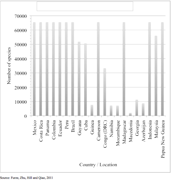
Figure I shows DZ8-10 with species numbers.
Figure II. Species-Area relations of locations

The gradient of the straight line plotted in Figure II is as follows:
![]() (5)
(5)
Hence (3) for the regression line is defined as follows:
![]() (non-significant) (6)
(non-significant) (6)
The gradient of the linear regression line shows a positive relationship between area and species numbers, the correlation = 0.19 (non-significant P=0.05).
The Species-Area relationship in Figure II can be written as:
![]() (non-significant) (7)
(non-significant) (7)
Figure III. GTOPO30 Enhanced Digital Elevation Model of Guyana, South America (1km resolution)

Figure IV. Quarterly mean precipitation (1961-90) of Guyana, South America (18.5 km resolution)

Guyana is illustrated in the DEM of Figure III. Guyana is between latitude 60° – 55° West, longitude 0° –7.5° North with elevation from 0 – 1500 metres above sea level. Sea level is shown in blue, low elevation is in dark green and low-medium elevation in lighter green to white.
Figure IV shows example data, where Guyana mean precipitation is 0.75 (January, April, July) 0–100 kg m2 to 200–300 kg m2 , and 0.25 (October) 0–100 kg m2 to 300–400 kg m2 . The quantity of precipitation is shown from low (dark blue) to high (dark red).
Figures III and IV provide examples of the data which was used to construct the fuzzy conditional algorithm for E2, Guyana which may be stated as follows:
![]() (8)
(8)
Where antecedent A1 represents mean temperature, A2 represents mean precipitation, A3 represents mean ground frost frequency, A4 represents altitude, consequent B represents the number of individual plant species occurrences and E2 represents the stress tolerant-ruderal plant strategy of the plant species present. (8) translates into the following conditions
IF Variables A =
• Temperature = 80–100% to 80–100% (A1(5))
• Precipitation = 0.75 A2 0–100 kg m2(A2(1)) to 200–300 kg m2
(A2(3)), 0.25 A2 0–100 kg m2 (A2(1)) to 300–400 kg m2(A2(4))
• Ground Frost frequency = 0–6 days to 0–6 days (A3(1))
• Altitude = –30–1,366 m (A4(1)) to 1,366–1,500 m (A4(2))
THEN B(51847)= E2
Temperature and ground frost frequency can be found on the IPCC web site.
Example locations of E1, E2, E3, E4, E5, E6 and E7 were defined using the control algorithmic structure shown in (4) as shown in Table III.
Table III. Categorisation of environments and plant life-history strategies
| Environment | Plant life-history strategy | Example location / number of individuals |
| 1 | R | Ecuador / 51857 – 65535 |
| 2 | S-R | Guyana / 50700 – 51847 |
| 3 | S-R / C-R | Cuba / 33356 – 50700 |
| 4 | C-R / C | Democratic Republic of the Congo / 11355 – 33366 |
| 5 | C-S-R / C-S | Georgia / 8805 – 11355 |
| 6 | C-S | Guinea / 2203 – 8805 |
| 7 | S | Macedonia / 0 – 2203 |
Source: Furze et al., 2013a
Where R represents ruderal, S-R represents stress tolerant-ruderal, C-R represents competitive-ruderal, C represents competitive, C-S-R represents competitive-stress tolerant-ruderal, C-S represents competitive-stress tolerant and S represents stress tolerant.
The root algorithm of (8) may be expanded to give ten separately weighted rules as follows:
1 If (temperature is high) and (GFF is low) then (strategy is S-R) (1)
2 If (precipitation is low) then (strategy is S-R) (0.75)
3 If (precipitation is low-medium) then (strategy is S-R) (0.75)
4 If (precipitation is medium) then (strategy is S-R) (0.75)
5 If (precipitation is low) then (strategy is S-R) (0.25)
6 If (precipitation is low-medium) then (strategy is S-R) (0.25)
7 If (precipitation is medium) then (strategy is S-R) (0.25)
8 If (precipitation is medium-high) then (strategy is S-R) (0.25)
9 if (altitude is low) then (strategy is S-R) (1)
10 If (altitude is low-medium) then (strategy is S-R) (1)
The rule set feeds into a fuzzy inference engine and results in an efficient surface area.
Figure V. Three-dimensional surface view for differentiation of plant strategy environment 2

In Figure V µ is given as the membership grade of each of the variables required to ordinate plant strategies. The surface algorithm shows the efficiency of the water-energy dynamic to be used in ordination of plant strategies as the input variable mean ground frost frequency is not used to ordinate the strategy here.
Dispersal of the plant strategy elements given in Table II using the input variables of mean temperature as objective 1 and mean precipitation as objective 2 is shown in Figure VI.
Figure VI. Plant strategy evolutionary strength Pareto

The utopia line and quadratic curve allow summarization of the distributions subject to the error of each expression. The water energy dynamic affords a binomial distribution of the strategy elements. The axis ‘objective 1’ (mean temperature, x) and ‘objective 2’ (mean precipitation, y) are n objective functions which may be expressed as Z in the following:
![]() (9)
(9)
Where vectors of Z are the average values of the elements dispersed in Figure VI, which are within the relational matrix multiplied by the number of objectives.
The utopia line and curve enable formation of further rules, which represent the function of the water energy dynamic.
Table IV. Utopia rules of plant strategy elements.
|
Rule |
Variables (3 significant figures) |
|||
|
∂1 |
∂2 |
∂3 |
||
|
1. |
-0.111 |
-0.154 |
0.541 |
|
|
2. |
0.014 |
0.014 |
0.007 |
0.03 |
Source: Own calculation, 2013
In the table ∂1 represents m in (2), ∂2 represents b in (2), ∂3 represents the third term of the quadratic curve,represents the residual error of the regressions. These expressions enable prediction of the modeled elements.
Conclusions
Variation in species numbers can not be explained by the increase in area, even when incorporating estimations of changes in environmental conditions (interpreted logarithmically from the intercept) and the rate of increase due to the species present (interpreted from the gradient of the regression line). An algorithmic approach is required to predict the number of species occurrences present in terms of groups of plant characteristics, with use of a T-S-K logic-based framework. Using a fuzzy logic approach enables categorization of species within 7 different environments according to the water-energy dynamic. Accurate and precise statements of ordination are obtained with use of high resolution data. Minimisation of antecedent variables enables further dispersal of strategy elements across combined objectives, enabling enhanced prediction of climatic variables and indeed of species occurrence numbers via linear and quadratic expressions of utopia. Distribution of species within areas of high biodiversity follow normal distribution, which enables further approximation of the characteristics of the species, following algorithmic approaches. Plant species environments range from 1 to 7 with ruderal strategy species existing in locations of highest species numbers through competitive to stress tolerant species in more extreme environments. Environment 1 is characterized by moderately high temperatures and high rainfall, being ideal conditions for plant growth, as opposed to extreme environments, which have lower rainfall and comparatively higher temperatures (Furze et al., 2013b).
The implementation of logic-based mathematics adds strength to related interdisciplinary fields of plant characterisation (Furze et al., 2013c). Additionally modelling of climatic variables and the characters of plants modeled therein is enhanced in terms of accuracy and pattern distribution. Examples of the potential uses of this work include the finer scale structuring of phylogenetic trees, the patterning of prey-taxis relations (Grunewald, Spillner, Bastkowski, Bögershausen and Moulton, 2013; Huson, Dezulian, Klöpper, and Steel, 2004; Ma, Han, Tao and Wu, 2013) and measurement of quantitative trait loci such as those involved in biochemical pathways (Kearsey and Pooni, 1996 [ch. 8]; Kraft and Ackerly, 2010). There are many areas of research fundamental to protective policies. The accessibility of higher mathematics to related subject areas and therefore policy makers is an important element to emphasize, especially with regard to vulnerable locations and indigenous populations in locations such as Ecuador, which are under threat of development (Pappalardo, Marchi and Ferrarese, 2013). Identification and expression of elements within priority conservation areas under threat of destructive human activity is of increasing importance, given the nature of the activities and the immediate effect on the concentrated biodiversity.
Modelling of plant species occurrence is important due to the primary level of plants within trophic systems. As such plant characterisation modelling studies making use of climatic and topographical data within time series makes use of the state of evolution of plants to infer the state of the climate. Techniques employed in this study enable characterisation of plant metabolism (photosynthesis) and life-form distribution. Plants share relationships with climatic conditions both on local and global scales, hence the levels of species richness are finely balanced with the climatic conditions within both time and space. This is especially pertinent in areas of high biodiversity. Policy formation, including national and international initiatives such as the protection status of areas of high biodiversity, conservation practice and Millenium Development Goals towards sustainable communities are all strengthened by the use of the interdisciplinary approach presented here.
References
Arrhenius, O. (1921). Species and Area. Journal of Ecology, vol. 9, pp. 95-99.
Barthlott, W., Mutke, J., Rafiqpoor, D., Kier, G. and Kreft, H. (2005). Global Centers of Vascular Plant Diversity. Nova Acta Leopoldina NF, vol. 92, pp. 61–83.
Bhattarai, K. R. and Vetaas, O. R. (2003). Variation in plant species richness of different life forms along a subtropical elevation gradient in the Himalayas, east Nepal. Global Ecology and Biogeography, vol. 12, pp. 327-340.
Furze, J., Zhu, Q.M., Qiao, F. and Hill, J. (2011). Species area relations and information rich modelling of plant species variation. Proceedings of the 17th International Conference on Automation and Computing (ICAC), 10 September, 2011, pp.63–68, http://ieeexplore.ieee.org/stamp/stamp.jsp?tp=&arnumber=6084902&isnumber=6084889
Furze, J. N., Zhu, Q. M., Qiao, F. and Hill, J. (2013a). Linking and implementation of fuzzy logic control to ordinate plant strategies. International Journal of Modelling, Identification and Control, vol. 19, pp. 333-342. DOI: 10.1504/IJMIC.2013.055651
Furze, J. N., Zhu, Q., Qiao, F. and Hill, J. (2013b). Implementing stochastic distribution within the utopia plane of primary producers using a hybrid genetic algorithm. International Journal of Computer Applications in Technology, vol. 47, pp. 68-77. DOI: 10.1504/IJCAT.2013.054303
Furze, J. N., Zhu, Q., Qiao, F. and Hill, J. (2013c). Mathematical methods to quantify and characterise the primary elements of trophic systems. International Journal of Computer Applications in Technology, vol. 47, pp. 315-325. DOI: 10.1504/IJCAT.2013.055324
Grunewald, S., Spillner, A., Bastkowski, S., Bögershausen, A. and Moulton, V. (2013). SuperQ: Computing Supernetworks from Quartets. IEEE/ACM Transactions on Computational Biology and Bioinformatics, vol. 10, pp. 151-160.
Hawkins, B. A., Field, R., Cornell, H. V., Currie, D. J., Guégan, J. F., Kaufman, D. M., Kerr, J. T., Mittelbach, G. G., Oberdorff, T., O’Brien, E. M., Porter, E. E. and Turner, J. R. G. (2003). Energy, water, and broad-scale geographic patterns of species richness. Ecology, vol. 84, pp. 3105-3117.
Hodgson, J. G., Wilson, P. J., Hunt, R., Grime, J. P., and Thompson K. (1999). Allocating C-S-R plant functional types: a soft approach to a hard problem. Oikos, vol. 85, pp. 282–294.
Humboldt, A. V. (1806). Ideen zu einer physiognomik der gewächse. Tübingen.
Humboldt, A. V. (1808). Ansichten der natur mit wissenschaftlichen erläuterungen. Tübingen.
Huson, D., Dezulian, T., Klöpper, T. and Steel, M. (2004). Phylogenetic Super-Networks from Partial Trees. IEEE/ACM Transactions on Computational Biology and Bioinformatics, vol. 1, pp. 151-158.
Jetz, W., Kreft, H., Ceballos, G., and Mutke, J. (2009). Global associations between terrestrial producer and vertebrate consumer diversity. Proceedings of the Royal Society B, vol. 276, pp. 269-278.
Kearsey, M. J. and Pooni, H. S. (1998). The genetical analysis of quantitative traits. London, UK. Chapman & Hall.
Kraft, N. J. B. and Ackerly, D. D. (2010). Functional trait and phylogenetic tests of community assembly across spatial scales in an Amazonian Forest. Ecological Monographs, vol. 80, pp. 401-422, 2010.
Ma, M., Han, Z., Tao, J. and Wu, D. (2013). A food chain model with prey-taxis and chemotaxis. International Journal of Modelling, Identification and Control, vol. 19, pp. 235-247.
Mitchell, T.D. and Jones, P.D. (2005). An improved method of constructing a database of monthly climate observations and associated high resolution grids. International Journal of Climatology, vol. 25, pp.693–712.
New, M., Hulme, M. and Jones, P. (1999). Representing twentieth century space-time climate variability. Part I-Development of a 1961–90 mean monthly terrestrial climatology. Journal of Climate, vol. 12, pp.829–856.
Niu, S., Yuan, Z., Zhang, Y., Liu, W., Zhang, L., Huang J. and Wan, S. (2005). Photosynthetic responses of C3 and C4 species to Water availability and competition. Journal of Experimental Botany, vol. 56, pp. 2867-2876.
Pappalardo, S. E., Marchi, M. D. and Ferrarese, F. (2013). Uncontacted Waorani in the Yasuní Biosphere Reserve: Geographical validation of the Zona Intangible Tagaeri Taromenane (ZITT). Plos One, vol. 8, pp. 1-15.
Schultes, R. E. and Reis, S. V. (Eds). (1997). Ethnobotany evolution of a discipline. Oregon, USA. Dioscorides Press.
Wright, D. H. (1983). Species-energy theory: an extension of species energy theory, Oikos, vol. 41, pp. 496-506.
Yesson, C., Brewer, P. W., Sutton, T., Caithness, N., Pahwa, J. S., Burgess, M., Gray, W. A., White, R. J., Jones, A. C., Bisby, F. A. and Culham, A. (2007). How global is the global biodiversity information facility? Plos One, vol. 11, pp. 1-10.
Zadeh, L. A. (1965). Fuzzy sets. Information and Control, vol. 8, pp. 338-353.
.
This article was published on September 15th: International Day of Democracy, in Global Education Magazine.


